Next: Overview of the
Up: THE BASIC SYSTEM
Previous: Automatic scaling of
The recurrent network falls into the framework described by Rumelhart, Hinton
and Williams [4]. It may be viewed as a single
layer error propagation (back propagation) network, part of whose output is
fed back to the input after a single frame time delay. This is shown in
figure 1 where the external input,  , and the
state input,
, and the
state input,  , together form the input vector, the output vector being
composed of the external output,
, together form the input vector, the output vector being
composed of the external output,  , and the state output,
  .
In practice, the external output is not trained to classify the current input
vector,
.
In practice, the external output is not trained to classify the current input
vector,  , but that of n frames previously,
  . This is to
allow some forward context in the classification, backward context is already
available through the state vector. For most of these experiments, a four
frame delay was used which corresponds to 64ms.
. This is to
allow some forward context in the classification, backward context is already
available through the state vector. For most of these experiments, a four
frame delay was used which corresponds to 64ms.
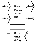
Figure 1: The recurrent network
The ``time-expansion'' or ``batch'' method of training recurrent networks is
adopted for computational efficiency reasons. After 32 frames on each of the
64 transputers, the actual outputs are compared with the desired outputs and
the contribution of these patterns to the gradient of the cross-entropy cost
function is computed. Cross-entropy is used both because of the
interpretation of the output units as probabilities and because it is found
to reduce the training time needed.
An adaptive step size algorithm was necessary to achieve training in
reasonable time. Each weight has a step size associated with it and the
weight is changed by this amount in the direction of the locally computed
gradient. If this gradient agrees in sign with the gradient when smoothed
with a first order filter over the whole of the training set, then the step
size is increased, otherwise it was decreased. In most experiments, the
increase was multiplication by a factor of 1.116 and the decrease was a
factor of 0.9. In two cases, pzc and pow, this proved to be
unstable, and increases of 1.1155 and 1.113 were used, respectively.
For the majority of the work presented in this paper, 96 state nodes were
used, which yields about 20,000 weights to be trained. 32 passes through the
training set were found to be sufficient and this could be achieved in 17
hours on the transputer array.
Next: Overview of the
Up: THE BASIC SYSTEM
Previous: Automatic scaling of