Shorten supports two forms of linear prediction: the standard  th
order LPC analysis of equation 1; and a restricted form
whereby the coefficients are selected from one of four fixed polynomial
predictors.
th
order LPC analysis of equation 1; and a restricted form
whereby the coefficients are selected from one of four fixed polynomial
predictors.
In the case of the general LPC algorithm, the prediction coefficients,
 , are quantised in accordance with the same Laplacian distribution
used for the residual signal and described in section 3.3.
The expected number of bits per coefficient is 7 as this was found to be
a good tradeoff between modelling accuracy and model storage. The
standard Durbin's algorithm for computing the LPC coefficients from the
autocorrelation coefficients is used in a incremental way. On each
iteration the mean squared value of the prediction residual is
calculated and this is used to compute the expected number of bits
needed to code the residual signal. This is added to the number of bits
needed to code the prediction coefficients and the LPC order is selected
to minimise the total. As the computation of the autocorrelation
coefficients is the most expensive step in this process, the search for
the optimal model order is terminated when the last two models have
resulted in a higher bit rate. Whilst it is possible to construct
signals that defeat this search procedure, in practice for speech
signals it has been found that the occasional use of a lower prediction
order results in an insignificant increase in the bit rate and has the
additional side effect of requiring less compute to decode.
, are quantised in accordance with the same Laplacian distribution
used for the residual signal and described in section 3.3.
The expected number of bits per coefficient is 7 as this was found to be
a good tradeoff between modelling accuracy and model storage. The
standard Durbin's algorithm for computing the LPC coefficients from the
autocorrelation coefficients is used in a incremental way. On each
iteration the mean squared value of the prediction residual is
calculated and this is used to compute the expected number of bits
needed to code the residual signal. This is added to the number of bits
needed to code the prediction coefficients and the LPC order is selected
to minimise the total. As the computation of the autocorrelation
coefficients is the most expensive step in this process, the search for
the optimal model order is terminated when the last two models have
resulted in a higher bit rate. Whilst it is possible to construct
signals that defeat this search procedure, in practice for speech
signals it has been found that the occasional use of a lower prediction
order results in an insignificant increase in the bit rate and has the
additional side effect of requiring less compute to decode.
A restrictive form of the linear predictor has been found to be useful.
In this case the prediction coefficients are those specified by fitting
a order polynomial to the last data points, e.g. a line to the
last two points:
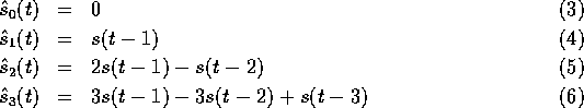
Writing  as the error signal from the
  th polynomial predictor:
As can be seen from equations 7-10 there is an efficient recursive algorithm for computing the set of polynomial prediction residuals. Each residual term is formed from the difference of the previous order predictors. As each term involves only a few integer additions/subtractions, it is possible to compute all predictors and select the best. Moreover, as the sum of absolute values is linearly related to the variance, this may be used as the basis of predictor selection and so the whole process is cheap to compute as it involves no multiplications.
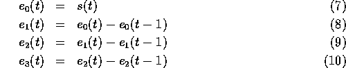
Figure 1 shows both forms of prediction for a range of maximum predictor orders. The figure shows that first and second order prediction provides a substantial increase in compression and that higher order predictors provide relatively little improvement. The figure also shows that for this example most of the total compression can be obtained using no prediction, that is a zeroth order coder achieved about 48% compression and the best predictor 58%. Hence, for lossless compression it is important not to waste too much compute on the predictor and to to perform the residual coding efficiently.